An Introduction to Bayesian Statistics
Bayesian statistics has emerged as a powerful methodology for making decisions from data in the applied sciences.

Complete the form below to unlock access to ALL audio articles.
What is Bayesian statistics?
In the ever-evolving toolkit of statistical analysis techniques, Bayesian statistics has emerged as a popular and powerful methodology for making decisions from data in the applied sciences. Bayesian is not just a family of techniques but brings a new way of thinking to statistics, in how it deals with probability, uncertainty and drawing inferences from an analysis. Bayesian statistics has become influential in physics, engineering and the medical and social sciences, and underpins much of the developing fields of machine learning and artificial intelligence (AI). In this article we will explore key differences between Bayesian and traditional frequentist statistical approaches, some fundamental concepts at the core of Bayesian statistics, the central Bayes’ rule, the thinking around making Bayesian inferences and finally explore a real-world example of applying Bayesian statistics to a scientific problem.
Bayesian vs frequentist statistics
The field of statistics is rooted in probability theory, but Bayesian statistics deals with probability differently than frequentist statistics. Frequentist thinking follows that the probability of an event occurring can be interpreted as the proportion of times the event would occur in many repeated trials or situations. By contrast, the Bayesian approach is based on a subjective interpretation of probability, where the probability of the event occurring relates to the analyst expressing their own evaluation as well as what happens with the event itself, and prior evidence or beliefs are used to help calculate the size of the probability. In essence, the Bayesian and frequentist approaches to statistics share the same goal of making inferences, predictions or drawing conclusions based on data but deal with uncertainty in different ways.
In practice, this means that, for frequentists, parameters (values about a population of interest that we want to estimate such as means or proportions) are fixed and unknown, whereas for Bayesians these parameters can be assigned probabilities and updated using prior knowledge or beliefs. In frequentist statistics, confidence intervals are used to quantify uncertainty around estimates, whereas Bayesian statistics provides a posterior distribution, combining the prior beliefs and likelihood of the data. P-values are used in frequentist statistics to test a hypothesis by evaluating the probability of observing data as extreme as what was observed, whereas Bayesian hypothesis testing is based on comparing posterior probabilities given the data, incorporating prior beliefs and updating them.
Bayesian fundamentals and Bayes’ rule
There are several concepts that are key to understanding Bayesian statistics, some of which are unique to the field:
- Conditional probability is the probability of an event A given B, which is important for updating beliefs. For example, a researcher may be interested in the conditional probability of developing cancer given a particular risk factor such as smoking. We extend this to Bayesian statistics and update beliefs using Bayes’ rule, alongside the three fundamental elements in a Bayesian analysis; the prior distribution, likelihood and posterior distribution.
- Prior distribution is some reasonable belief about the plausibility of values of an unknown parameter of interest, without any evidence from the new data we are analysing.
- Likelihood encompasses the different possible values of the parameter based on analysis of the new data.
- Posterior distribution is the combination of the prior distribution and the likelihood using Bayes’ rule:
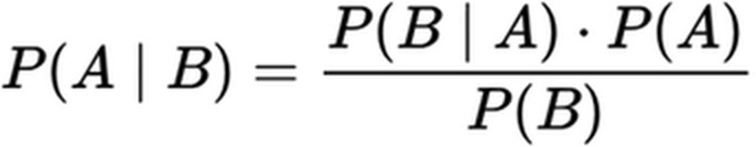
where A and B are some unknown parameter of interest and some new data, respectively. P(A|B) is the probability of A given B is true or the posterior distribution, P(B|A) is the probability of B given A is true or the likelihood, and P(A) and P(B) are the independent probabilities of A and B.
This process of using Bayes’ rule to update prior beliefs is called Bayesian updating. The information we aim to update can also be simply known as the prior. It is important to note that the prior can take the form of other data, for example a statistical estimate from a previous analysis, or simply an estimate based on belief or domain knowledge. A prior belief need not be quantifiable as a probability, but in some cases may be qualitative or subjective in nature, for example a doctor’s opinion on whether a patient had a certain disease before a diagnostic test is conducted. After updating the prior using Bayes’ rule, the information we end up with is the posterior. The posterior distribution forms the basis of a statistical inference made from a Bayesian analysis.
Example of Bayesian statistics
Let us consider an example of a simple Bayesian analysis, where rather than go through equations in detail, we use graphs to illustrate the prior distribution, likelihood and posterior distribution under a beta distribution. The beta distribution is commonly used (in both Bayesian and frequentist statistics) in estimating the probability of an outcome, where this probability can take any value between 0 and 1 (0% and 100%).
Suppose we are conducting a survey in rural Nigeria where we collect responses from participants to estimate the prevalence of visual impairment in an elderly community. First, we need to define our prior distribution, which we do using the prior belief that the prevalence will be 75% based on previous surveys on visual impairment among similarly aged participants. Our prior distribution is then centered around 75% (Figure 1.1). Next, we observe in the current survey that 85% of participants have visual impairment, and so our likelihood is centered around this value (Figure 1.2). Likelihood is calculated using the Bernoulli distribution, a distribution used specifically for modeling binary outcomes or events (visual impairment: yes/no) in this example, for the analysis of our current data, compared with Beta distribution for the prior which differs in nature in that it is an expression of a prior belief.
After setting up the prior and computing the likelihood, we next combine them and calculate the posterior distribution using Bayes’ rule. In our example, we find that the posterior distribution (based on the Beta distribution) has been influenced by our prior belief and moved to a value less than that which we observed in the current survey data with a mode at around 80% (Figure 1.3).
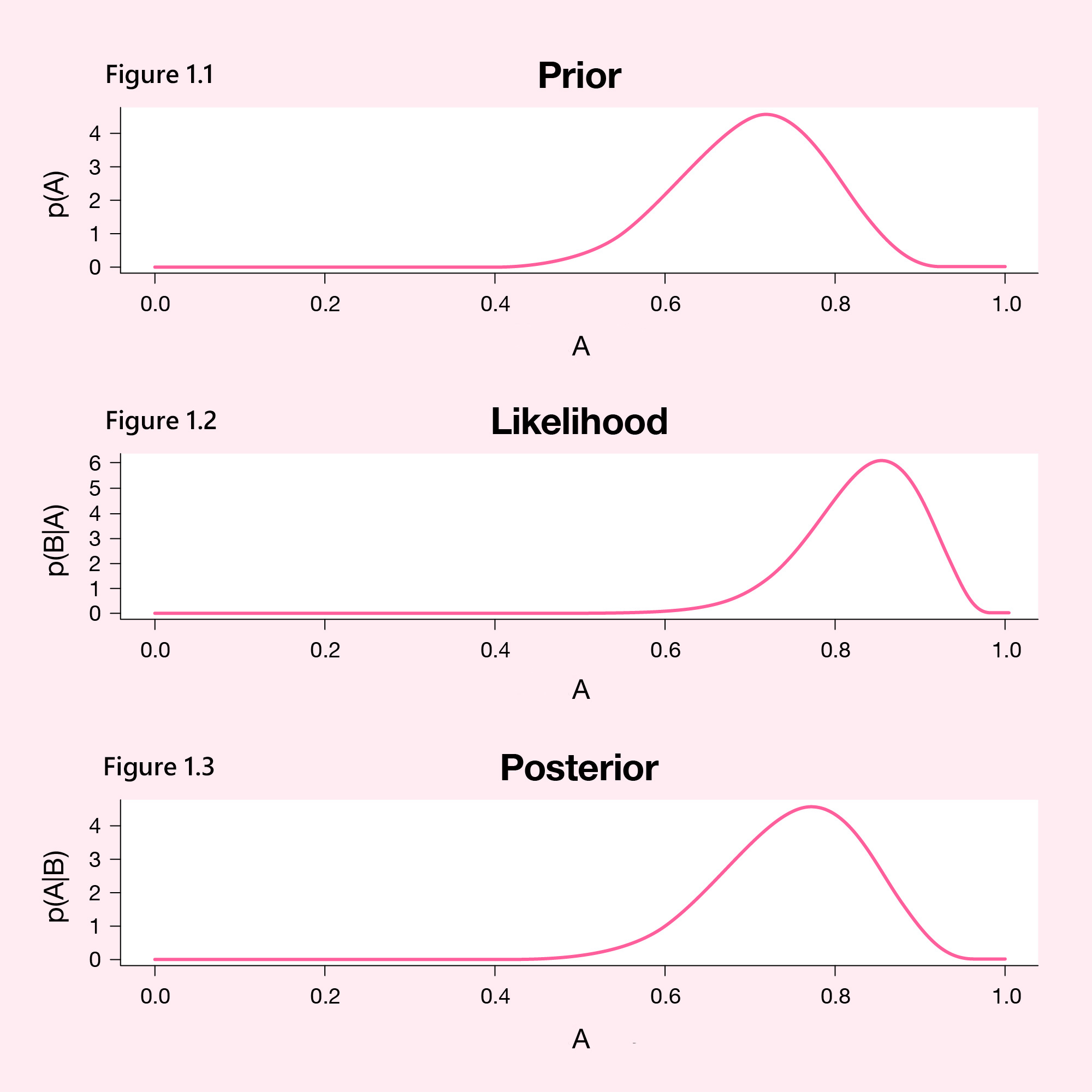
Figure 1: Bayesian distributions for prevalence of visual impairment.
Where A is the unknown parameter for which probabilities can be calculated, and
B is the new data.
An important aspect of this type of analysis is that the posterior distribution is heavily influenced by the number of participants in our current study. If we imagined that our current survey had a much higher sample size, the posterior distribution may not have moved away from 85% at all. As more new data are collected, the likelihood begins to dominate the prior. This example shows the key fundamentals of Bayesian inference in action and demonstrates how we can use Bayesian inference to update our beliefs based on new data.